Tutorial

Object Detection with YOLOv8 Advanced Capabilities

Updated on April 10, 2025

Technical Writer

Object Detection with YOLOv8 Advanced Capabilities

Introduction

YOLO is a state-of-the-art object detection algorithm. Due to its processing power, it has become almost a standard way of detecting objects in computer vision. Earlier, people used techniques like sliding windows, RCNN, fast RCNN, and faster RCNN for object detection.

But in 2015, YOLO (You Only Look Once) was invented, and this algorithm and its successors began outperforming all others.

In this article, we explore Ultralytics’ YOLOv8, a powerful real-time object detection and image segmentation model. Built on the latest advancements in deep learning and computer vision, YOLOv8 offers impressive speed and accuracy. Its sleek architecture supports a broad spectrum of applications and can effortlessly be adapted to various hardware platforms—from edge devices to cloud-based APIs—through the user-friendly Ultralytics Python package.

YOLO is a state-of-the-art (SOTA) object detection algorithm, and it is so fast that it has become one of the standard ways of detecting objects in the field of computer vision. Previously, sliding window operations were most common in object detection. Then came improvements, and faster versions of object detection were introduced, such as CNN, R-CNN, Fast RCNN, and many more.

We will explore the incredible capabilities of YOLOv8, a state-of-the-art model for object detection. Our focus will be on its features and the advancements it brings. Additionally, we will discuss how to implement YOLOv8 with a custom dataset seamlessly while also examining the evolution of the YOLO series and the challenges and limitations faced in developing previous versions of YOLO.

Prerequisites

Python Programming: Basic knowledge of Python is essential for setting up and using YOLOv8.
Machine Learning Basics: Understanding fundamental ML concepts like supervised learning, neural networks, and training/evaluation metrics will be helpful.
Deep Learning Frameworks: Familiarity with PyTorch or TensorFlow, as YOLOv8 can be implemented using these frameworks.
Computer Vision Basics: Knowledge of image processing techniques, bounding boxes, and object detection concepts will aid in understanding YOLOv8.
CUDA and GPU Setup: A CUDA-capable GPU is recommended for faster training and inference, along with basic knowledge of configuring CUDA for deep learning.

Brief overview of object detection in computer vision

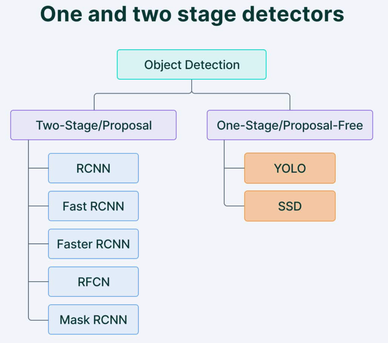
Object detection is the union of two computer vision sub-disciplines: object localization and image classification. It involves recognizing specific classes of objects (like humans, animals, or cars). Its primary aim is to create computational methods and models that answer a fundamental question in computer vision: the identification and location of objects. Object detection algorithms can be divided into two main categories: single-shot detectors and two-stage detectors.

This classification is based on the number of times the same input image is passed through a network.

Image Source

The key evaluation metrics for object detection are accuracy, classification, localization precision, and swiftness. Object detection serves as a base for many other computer vision tasks, such as segmentation, image captioning, object tracking, and more. Object detection is widely used in many real-world applications, such as autonomous driving, robot vision, video surveillance, etc. One of the recent examples is the object detection system in Tesla cars, which is designed to identify other vehicles, pedestrians, animals, road signs, lane markers, and any obstacles that the vehicle may encounter on the road.

In the below image, we can review the history of object detection and how far this technology has evolved from traditional object detection to deep learning-based detection.

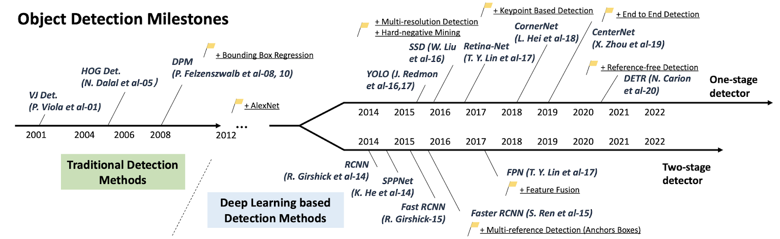
A road map of object detection. Milestone detectors in this figure: VJ Det., HOG Det., DPM, RCNN, SPPNet, Fast RCNN, Faster RCNN, YOLO, SSD, FPN, Retina-Net, CornerNet, CenterNet, DETR.

Introduction to YOLO (You Only Look Once) and its importance

YOLO was introduced in 2015 by R. Joseph (PJ Reddie) and stood out for its impressive speed, processing 155 frames per second with a mean average precision (mAP) of 52.7%. A later, more advanced version delivered improved accuracy with a mAP of 63.4% while running at 45 frames per second.

The YOLO approach diverges significantly from two-stage detectors by employing a single neural network on the entire image. This network segments the image into regions and predicts bounding boxes and probabilities for each region concurrently. This results in an increased speed during the detection process. Despite its significant enhancement in detection speed, YOLO experiences a decrease in localization accuracy compared to two-stage detectors, particularly in detecting small objects. YOLO’s subsequent versions have paid more attention to this problem.

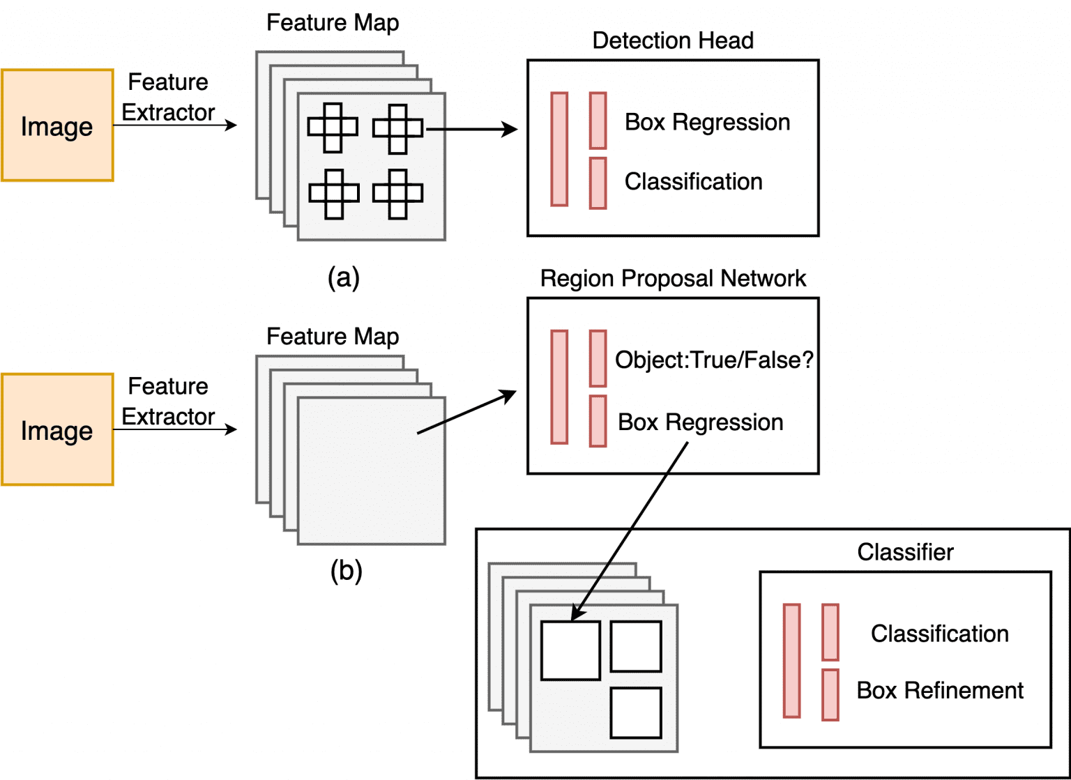
Single-shot object detection

Single-shot object detection swiftly analyzes entire images in one go to identify objects. However, it tends to be less accurate than other methods and might struggle with detecting smaller objects. Despite this, it’s computationally efficient and suitable for real-time detection in resource-limited settings. YOLO, a single-shot detector, employs a fully convolutional neural network for image processing.

Two-shot object detection

Two-shot or two-stage object detection involves employing two rounds of the input image to forecast the existence and positioning of objects. The initial round generates a series of proposals or potential object locations, while the subsequent round enhances these proposals to make conclusive predictions. While more precise than single-shot object detection, this method also incurs greater computational expense.

Applications in various domains

YOLO (You Only Look Once) has found various applications across different domains due to its real-time object detection capabilities. Some of its applications include:

Surveillance and Security: YOLO is used for real-time monitoring in surveillance systems, identifying and tracking objects or individuals in video streams Autonomous Vehicles: It’s employed in self-driving cars and autonomous systems to detect pedestrians, vehicles, and objects on roads, aiding in navigation and collision avoidance
Retail: YOLO can be used for inventory management, monitoring stock levels, and even for applications like smart retail shelves or cashier-less stores
Healthcare: It has potential in medical imaging for the detection and analysis of anomalies or specific objects in medical scans
Augmented Reality (AR) and Virtual Reality (VR): YOLO can assist in AR applications for recognizing and tracking objects or scenes in real time
Robotics: YOLO is used for object recognition and localization in robotics, enabling robots to perceive and interact with their environment more effectively
Environmental Monitoring: It can be applied in analyzing satellite images or drone footage for environmental studies, like tracking wildlife or assessing land use
Industrial Automation: YOLO can assist in quality control processes by identifying defects or anomalies in manufacturing lines

YOLO’s ability to perform real-time object detection with reasonably good accuracy makes it versatile for a wide range of applications that require swift and accurate object recognition.

How does YOLO work?

Let us assume we are working on an image classification problem and want to understand if the given image is of a person or a dog. In that case, the output of a neural network is simple. It will output one if a dog is present or 0 if no dogs are present in the image.

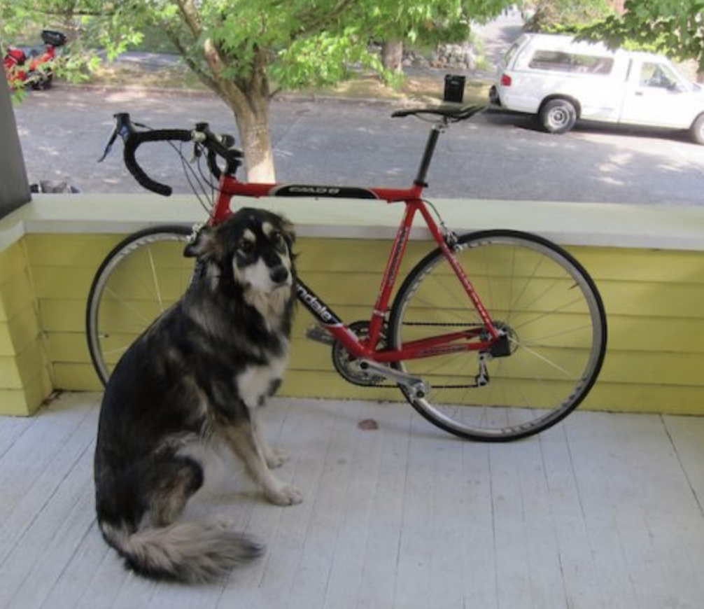
When we talk about object localization, the problem is not only the class but where the object is present in the image. This is done by drawing a bounding box or determining the position of the image within the image.

In short, the YOLO model is trained on labeled datasets, optimizing the model parameters to minimize the difference between predicted bounding boxes and ground-truth bounding boxes. With the help of bounding box coordinates and the class probability, we not only have the detected object but also the answer to object localization. Now, let’s get into more detail and break down what we just described.

The YOLO algorithm takes an image as an input and passes it to a deep Convolutional Neural Network. This neural network generates an output in the form of a vector that appears similar to this [Pc, bx, by, bw, bh, c1, c2, c3]. For convenience, let us denote this vector by n.

Pc is the probability of the class, which shows if an object is present or not.
bx, by, bw, bh specifies the coordinates of the bounding box from the center point of the object.
In image classification, the variables c1, c2, and c3 represent different classes present in the image. For example, if c1 corresponds to “dog,” then c1 will be equal to 1 when a dog is present, while all other classes will be 0. Similarly, if c2 represents “human,” then c2 will be set to 1 when a human is detected, with the remaining classes being 0. If no object is present in the image, the vector representing the classes will be [0, ?, ?, ?, …]. In this scenario, the probability score (Pc) will be 0, making the values of the other elements in the vector irrelevant.
This is fed to the neural network. Here, we have provided one example, but in the real world, many images are provided as the training set. These images are converted into vectors for each corresponding image. Since this is a supervised problem, the X_train and y_train will be the images and the vectors corresponding to the image, and the network will again output a vector.

This approach works for a single object in an image, but if there are multiple objects in a single image. It will be difficult to determine the dimension output of the neural network.

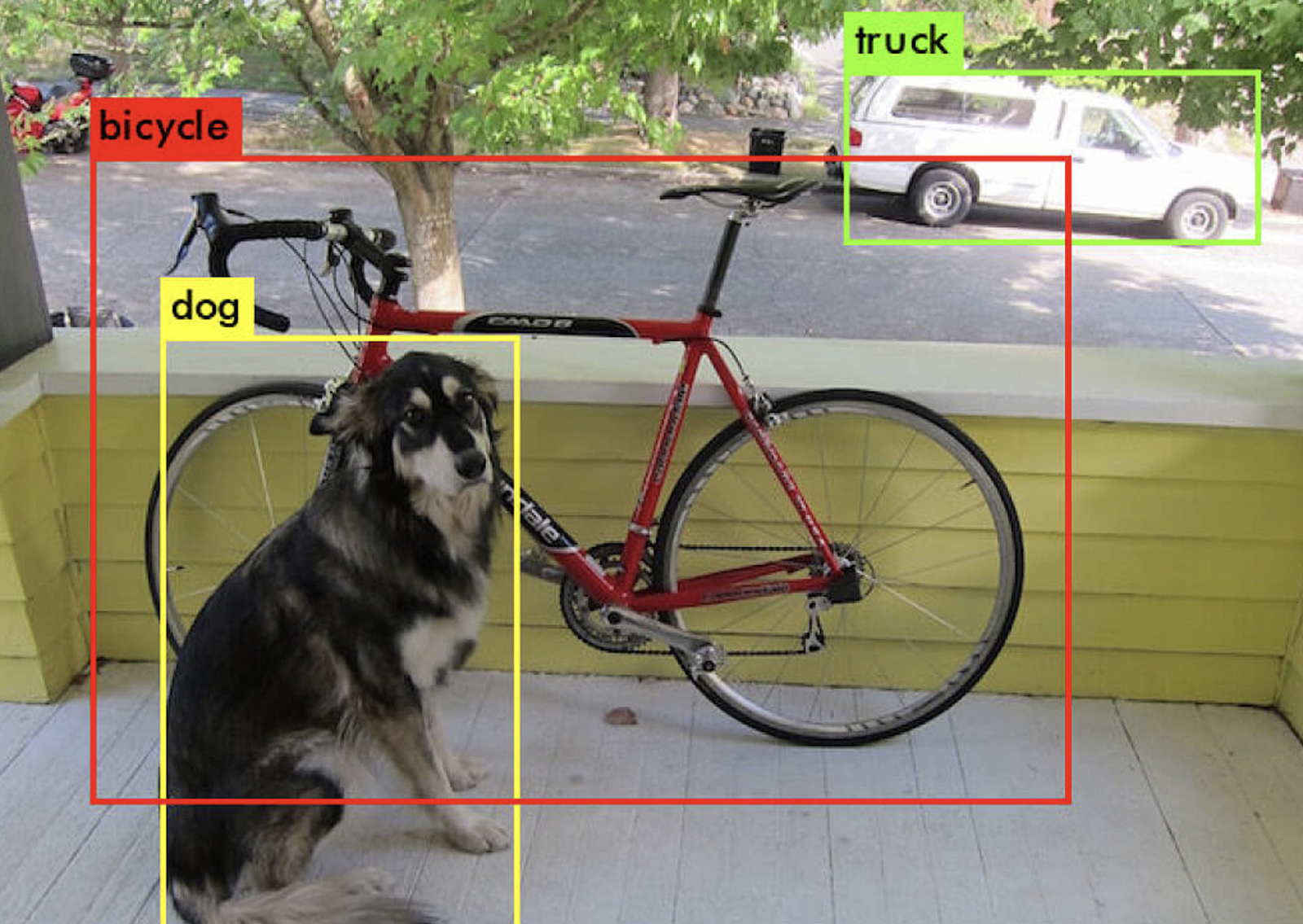
So, in this case, there are multiple objects with multiple bounding boxes in one image. YOLO will divide the image into S x S grid cells.

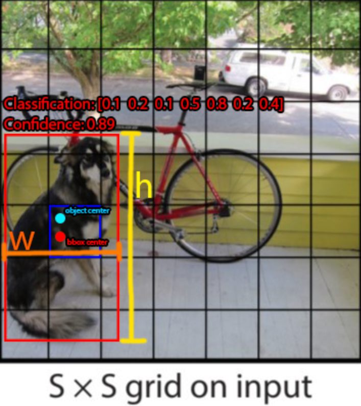
Here, every section of the grid is tasked with predicting and pinpointing the object’s class while providing a probability value. These are called Residual blocks.

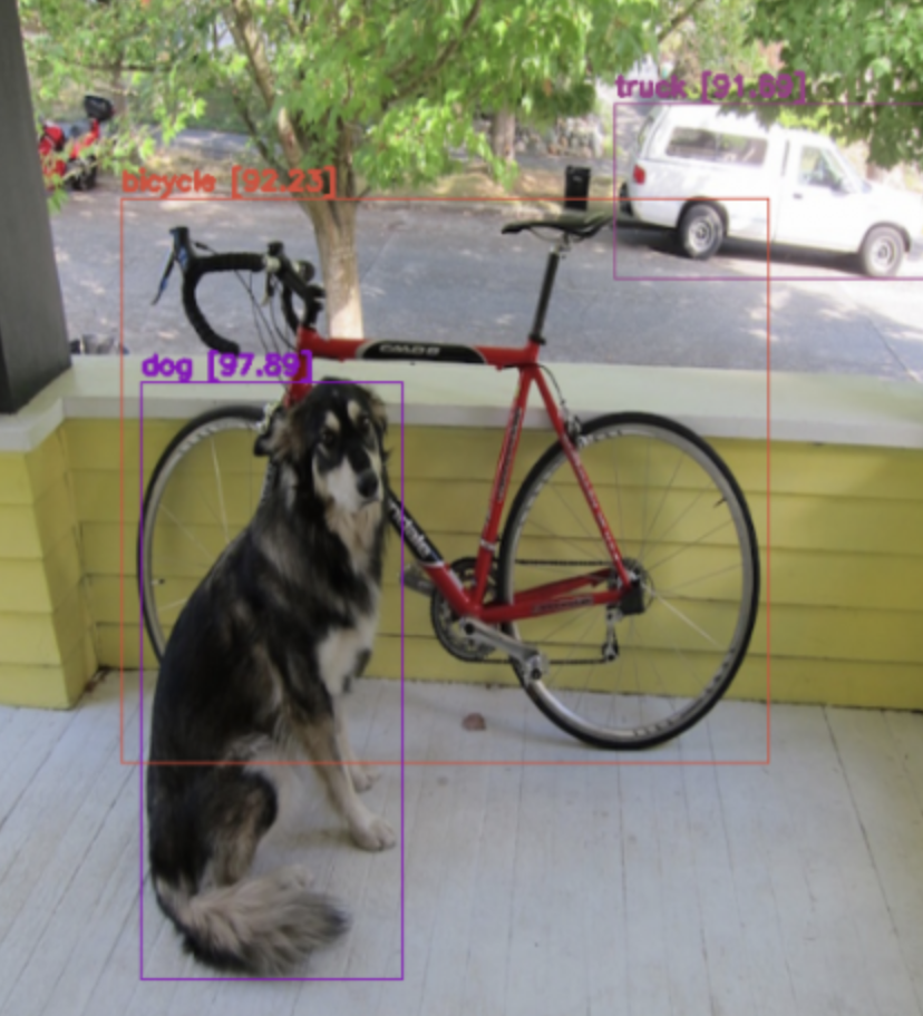
The next step is to find the Bounding box of the objects in the image. These bounding boxes corresponding to each object are the vectors that locate the object, as we discussed earlier. The attributes of the vector are n= [Pc, bx, by, bw, bh, c1, c2, c3]. YOLO will generate many of these bounding boxes for each potential object in the image and later filter these down to those with the highest prediction accuracy.

That means for one image, we will get S x S x n. This is because we have an S x S grid of cells, and each cell is a vector of size n. So now, with the image, we have the corresponding bounding box or rectangles that we can use as the training data set. Using this now, we can train our neural network and generate predictions. This is the basis of the YOLO algorithm. The name YOLO, or ‘You Only Look Once,’ is because the algorithm is not iterating over one image.

Even with this methodology, certain adjustments are necessary to enhance the accuracy of predictions. One issue that often comes up is detecting multiple bounding boxes or rectangles for one given object. Out of all the bounding boxes, only one is relevant.

Source

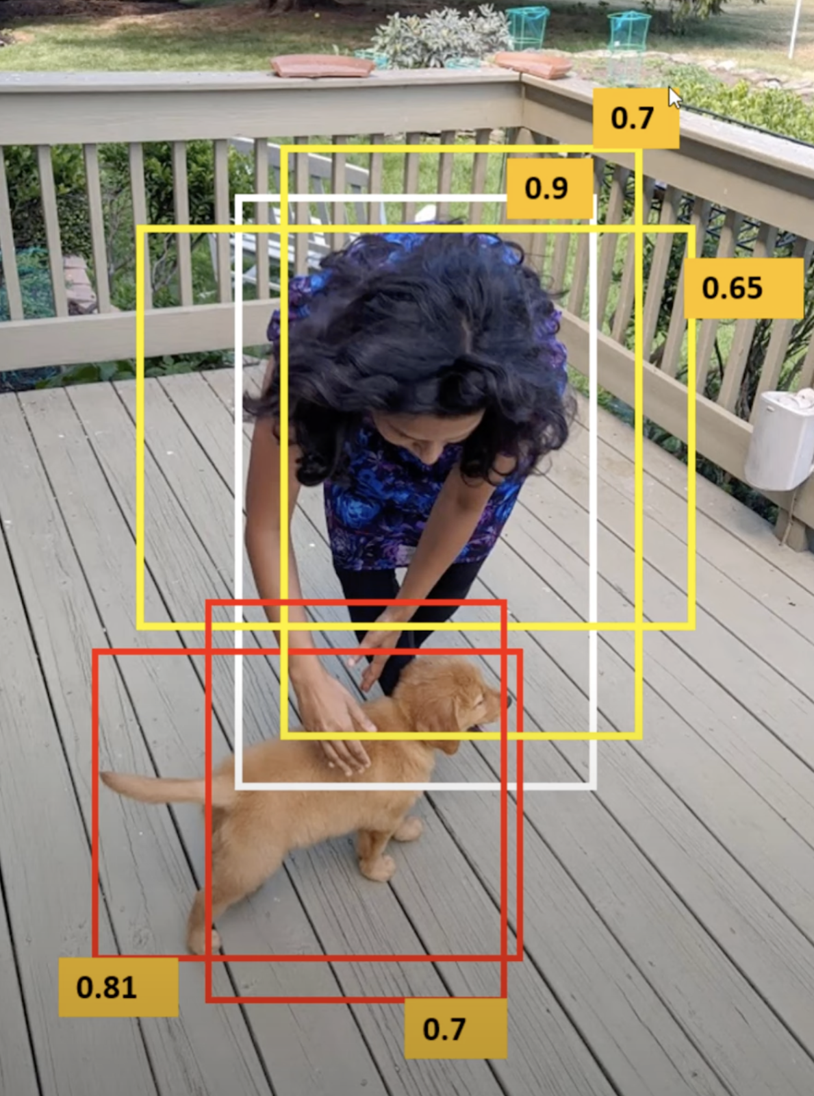
To tackle the multiple bounding box issue, the model uses the concept of IOU or intersections over unions, which has a value range of 0 to 1. The main aim of the IOU is to determine the most relevant box out of the multiple boxes.

IoU measures the overlap between a predicted bounding box and a ground truth bounding box. The value is calculated as the ratio of the area of overlap between these two bounding boxes to the total area encompassed by their union.

The formula for calculating IoU is:

IoU=Area of Overlap/Area of UnionIoU

Where:

Area of Overlap: The region where the predicted bounding box and the ground truth bounding box intersect
Area of Union: The total area encompassed by both the predicted bounding box and the ground truth bounding box

IoU values range from 0 to 1. A value of 1 indicates a perfect overlap between the predicted and ground truth bounding boxes, while a value of 0 means there is no overlap between the two boxes. In object detection, a higher IoU typically signifies better accuracy and precision in localizing objects within images.

The algorithm ignores the predicted value of the grid cell, which has a low IOU value.

Next, establishing a threshold for IoU alone may not suffice, as an object could potentially be associated with multiple bounding boxes surpassing the threshold value. Retaining all the boxes could introduce unwanted noise. Hence, calculating the Non-Maximum Suppression (NMS) becomes crucial, allowing the model to retain only those object-bounding boxes with the highest probabilities.

After getting these unique boxes, there could be another issue. What if a single cell contains two centers of objects? In this case, the grid cell can represent only one class. In such cases, Anchor Boxes can resolve the issue.

Source

Anchor boxes represent predetermined bounding boxes with specific height and width dimensions. These boxes are established to encompass the scale and proportions of particular object classes that one aims to detect, often selected according to the object sizes present within the training datasets.

This covers the basics of the YOLO algorithm. YOLO’s strength lies in its ability to detect objects in real-time, but due to its single-pass approach, it sometimes still struggles with small objects or closely packed objects in an image.

The evolution of YOLO models from YOLOv1 to YOLOv8

Image Source

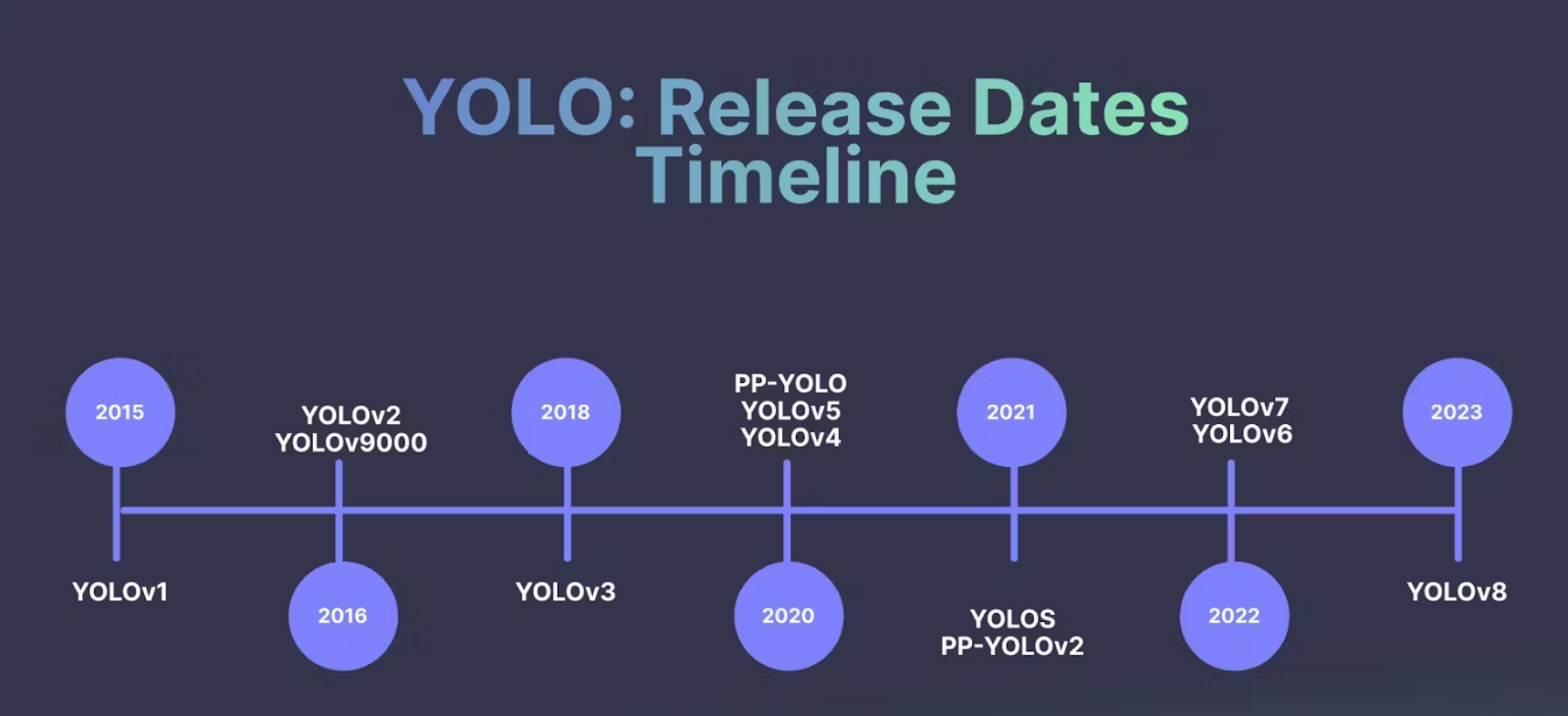
This section briefly overviews the YOLO framework’s evolution from YOLOV1 to YOLOv8. YOLO was introduced in a series of papers by Joseph Redmon and Ali Farhadi and has seen several iterations that have improved its speed, accuracy, and robustness.

YOLOv1 (2016): The first version of YOLO introduced a groundbreaking approach to object detection by framing it as a regression problem to spatially separated bounding boxes and associated class probabilities. YOLO divided the input image into a grid and predicted bounding boxes and class probabilities directly from the full image in a single pass, enabling real-time object detection.

YOLOv2 (2016): YOLOv2 improved on the original version by introducing various changes in the architecture. It included batch normalization, high-resolution classifiers, anchor boxes, etc., aiming to enhance speed and accuracy.

YOLOv3 (2018): In 2018, Joseph Redmon and Ali Farhadi published a paper on arXiv called YOLOv3: An Incremental Improvement. YOLOv3 further refined the architecture and training methods. It incorporated feature pyramid networks (FPN) and prediction across different scales to improve detection performance, especially for small objects. YOLOv3 also introduced multiple detection scales and surpassed previous versions’ accuracy.

YOLOv4 (2020): Alexey Bochkovskiy and others developed a new and improved version of YOLO, YOLOv4: Optimal Speed and Accuracy of Object Detection. YOLOv4 brought significant speed and accuracy improvements over its predecessor. This version focused on improving the network backbone. It incorporated various state-of-the-art techniques, such as the use of the CSPDarknet53 as the backbone, the Mish activation function, and the introduction of the weighted-Residual-Connections (WRC) as well as other novel approaches to augment performance. However, this was the year Joseph Redmon left computer vision research.

YOLOv5 (2020): In 2020, merely two months after the introduction of YOLOv4, Glenn Jocher, representing Ultralytics, unveiled YOLOv5. This release marked a significant stride in the YOLO series. YOLOv5, while not a direct iteration from the original YOLO creators, was a popular release from the open-source community. It optimized and simplified the architecture and introduced a focus on compatibility, making the model more accessible and easier to implement for various applications. YOLOv5 introduced a more modular and flexible architecture. The primary distinction with YOLOv5 was its development using PyTorch instead of DarkNet, the framework utilized in prior YOLO versions.

When tested on the MS COCO dataset test-dev 2017, YOLOv5x showcased an impressive AP of 50.7% using an image size of 640 pixels. With a batch size of 32, it can operate at 200 FPS on an NVIDIA V100. By opting for a larger input size of 1536 pixels, YOLOv5 can achieve an even greater AP of 55.8%.

Scaled-YOLOv4: In CVPR 2021, the authors of YOLOv4 introduced Scaled-YOLOv4. The primary innovation in Scaled-YOLOv4 involved the incorporation of scaling techniques, where scaling up led to a more precise model at the cost of reduced speed, while scaling down resulted in a faster model with a sacrifice in accuracy. The scaled-down architecture was called YOLOv4-tiny and worked well on low-end GPUs. The algorithm ran 46 FPS on a Jetson TX2 or 440 FPS on RTX2080Ti, achieving 22% mAP on MS COCO. The expanded model architecture known as YOLOv4-large encompassed three sizes: P5, P6, and P7. This architecture was specifically tailored for cloud GPU use and attained a cutting-edge performance, surpassing all preceding models by achieving a 56% mean average precision (mAP) on the MS COCO dataset.

YOLOR: YOLOR (You Only Learn One Representation) was developed in 2021 by the same research team that developed YOLOv4. A multi-task learning method was devised to create a unified model handling classification, detection, and pose estimation tasks by acquiring a general representation and employing sub-networks for task-specific data. YOLOR, designed akin to how humans utilize prior knowledge for new challenges, underwent an assessment on the MS COCO test-dev 2017 dataset, achieving an mAP of 55.4% and mAP50 of 73.3% while maintaining a speed of 30 FPS on an NVIDIA V100.

YOLOX (2021): YOLOX aimed to further improve speed and accuracy. It introduced the concept of Decoupled Head and Backbone (DHBB) and designed a new data augmentation strategy called “Cross-Stage Partial Network (CSPN) Distillation” to enhance performance on small objects.

YOLOv6: Published in the year 2022 by Meituan Vision AI Department YOLOv6: A Single-Stage Object Detection Framework for Industrial Applications YOLOv6-L achieved better accuracy performance (i.e., 49.5%/52.3%) than other detectors with a similar inference speed on an NVIDIA Tesla T4.

YOLOv7 (2022): The same authors of YOLOv4 and YOLOR published YOLOv7: Trainable bag-of-freebies sets new state-of-the-art for real-time object detectors. YOLOv7 introduces three key elements: E-ELAN for efficient learning, model scaling for adaptability, and a “bag-of-freebies” strategy for accuracy and efficiency. One aspect, re-parametrization, enhances model performance. The latest YOLOv7 model surpassed YOLOv4 by reducing parameters and computation significantly by 75% and 36%, respectively, while improving average precision by 1.5%. YOLOv7-tiny also reduced parameters and computation by 39% and 49% without compromising mean average precision (mAP).

DAMO-YOLO (2022): Alibaba Group published a paper titled DAMO-YOLO: A Report on Real-Time Object Detection Design. The document details various methods to enhance the accuracy of real-time video object detection. A novel detection backbone design derived from Neural Architecture Search (NAS) exploration, an extended neck structure, a more refined head structure, and the integration of distillation technology to enhance performance even further. These methods involved utilizing MAE-NAS for neural architecture search and implementing Efficient-RepGFPN inspired by GiraffeDet.

YOLOv8(2023): Recently we were introduced to YOLOv8 from the Ultralytics team. A full range of vision AI tasks, including detection, segmentation, pose estimation, tracking, and classification are supported by YOLOv8. This SOTA algorithm has higher mAPs and lower inference speed on the COCO dataset. However, the official paper is yet to be released.

What is new in YOLOv8

YOLOv8 is the latest version of YOLO in the object detection field. A few of the key updates in this version are:

A refined network architecture designed for enhanced performance and efficiency.
Revised Anchor boxes design: Anchor boxes have been restructured to optimize the detection of object scales and aspect ratios within specific classes.

These predefined bounding boxes are tailored to the sizes and variations of objects in training datasets, ensuring more accurate object localization and recognition in object detection models.

Adjusted loss function to improve overall accuracy in the predictions.
YOLOv8 integrates an adapted CSPDarknet53 backbone alongside a self-attention mechanism situated in the network’s head.

Architecture Overview of YOLOv8

The layout shown in the image was made by RangeKing on GitHub and is a great way of visualizing the architecture.

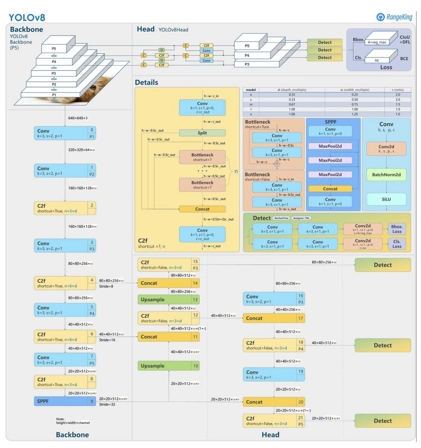
The major changes in the layout are:

New convolutions in YOLOv8
Anchor-free Detections
Mosaic Augmentation

For a more comprehensive explanation, we recommend referring to the earlier post, where the intricate details of the YOLOv8 architecture are thoroughly explained.

Benchmark Results Across YOLO lineage

The Ultralytics team has benchmarked YOLOv8 using the COCO dataset, revealing notable advancements compared to prior YOLO iterations across all five model sizes. The figure below compares YOLOv8 with the previous YOLO series.

Source

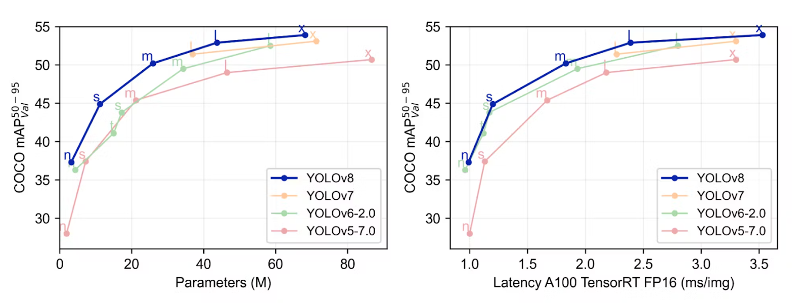
As mentioned in these sections, the below metrics were used to understand the model’s efficiency.

Performance (mAP)
Speed of the inference (In fps)
Compute the model size in FLOPs and params

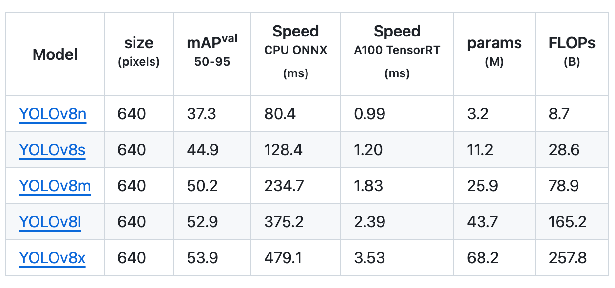
YOLOv8 accommodates various computer vision tasks, enabling the execution of object detection, image segmentation, object classification, and pose estimation. Each task serves a distinct purpose and caters to different objectives and use cases. Here are the benchmarking results of 5 YOLOv8 models.

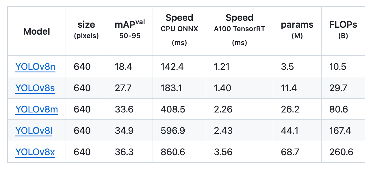
Detection

Object detection involves identifying the location and class of objects in an image or video stream.

In comparing object detection across five different model sizes, the YOLOv8m model obtained a mean Average Precision (mAP) of 50.2% on the COCO dataset. Meanwhile, the YOLOv8x, the largest model among the set, achieved 53.9% mAP despite having more than twice the number of parameters.

Using the Open Image v7 dataset, the YOLOv8x model obtained an mAP of 36.3% with almost the same number of parameters.

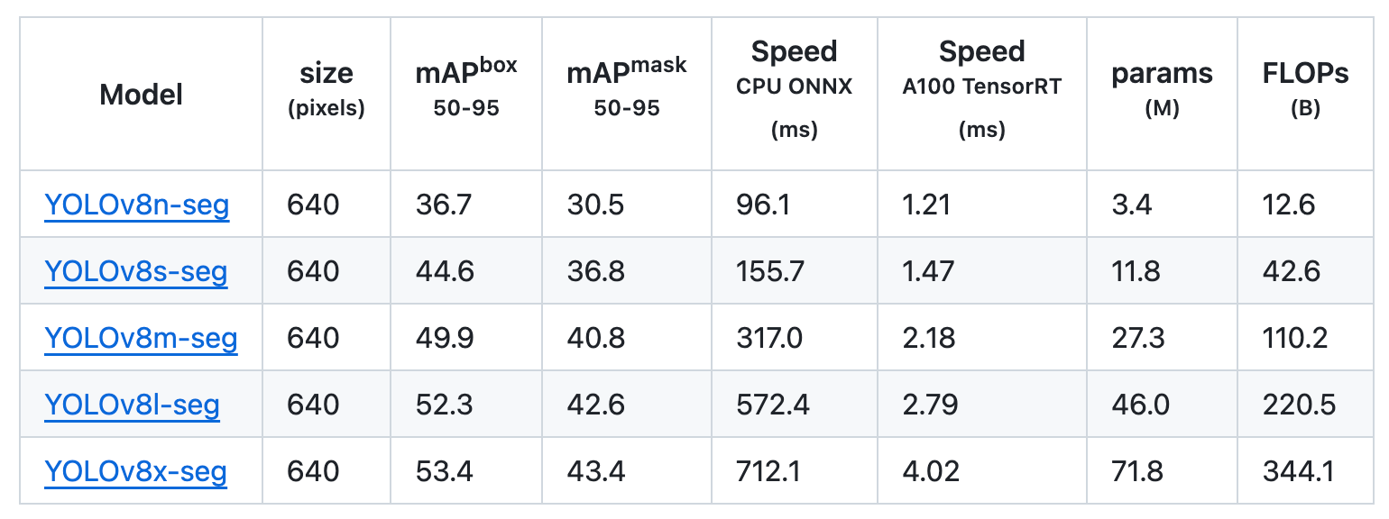
Segmentation

Instance segmentation in object detection involves identifying individual objects in an image and segmenting them from the rest of the image.

For object segmentation, these models were trained on COCO-Seg, which included 80 pre-trained classes.

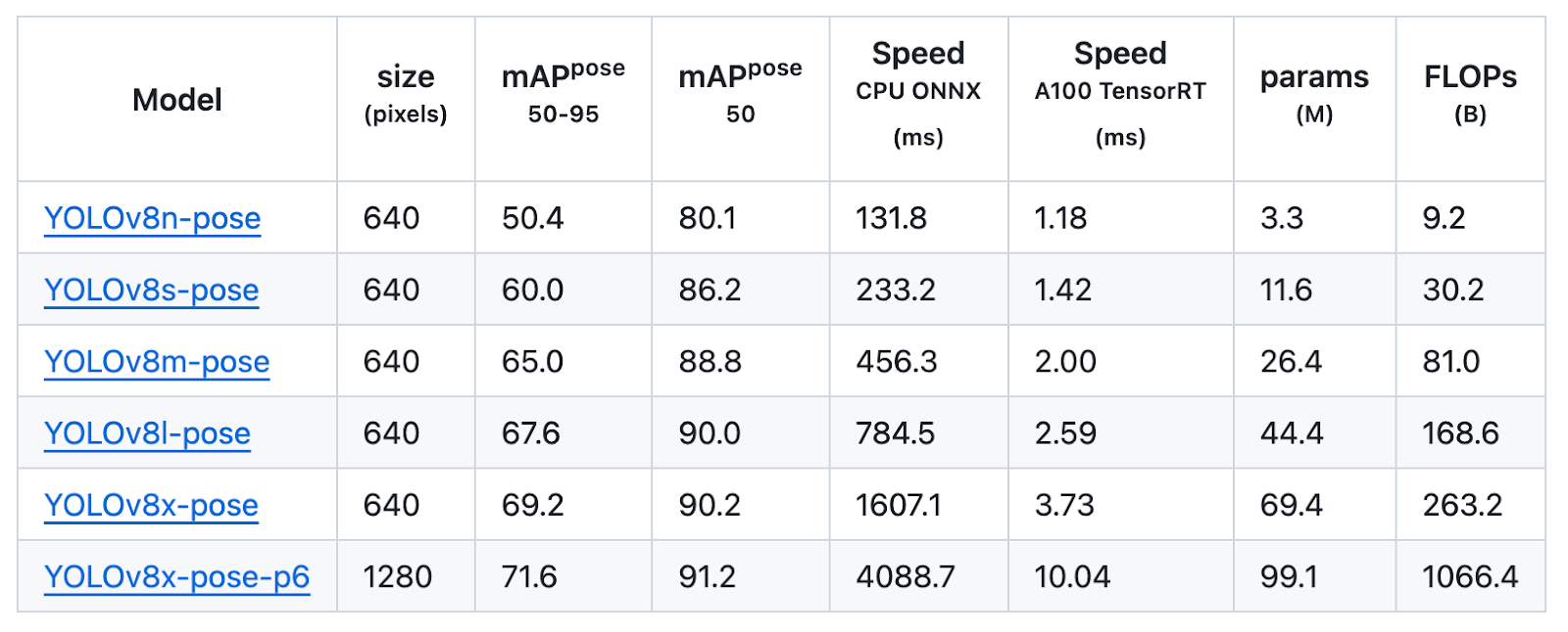
Pose

Pose estimation is the process of identifying key points within an image, commonly known as key points, and determining their specific locations.

These models trained on COCO-Pose included one pre-trained class, a person.

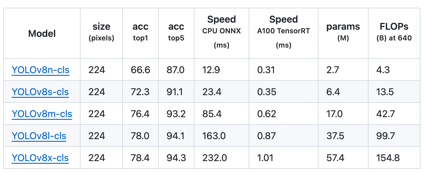
Classification

Classification is the simplest of the other tasks and involves classifying an entire image into one of a set of predefined classes. An image classifier produces a singular class label accompanied by a confidence score.

These models were trained on ImageNet, which included 1000 pre-trained classes.

Due to its exceptional accuracy and performance, YOLOv8 can be a great choice for any computer vision project.

Code Demo

In this article, we will walk through the steps to implement YOLOv8. Please follow the step-by-step process to get a better understanding. YOLOv8 is highly efficient and can be accelerated significantly by utilizing the computational power of a GPU. The YOLOv8n model can easily be trained on a Free GPU.

Installing Ultralytics to work with yolov8 and import the necessary libraries.

!pip install ultralytics

#Import necessary Libraries
from PIL import Image
import cv2
from roboflow import Roboflow
from ultralytics import YOLO
from PIL import Image

Constructing a personalized dataset can be a tedious task, demanding numerous hours to gather images, annotate them accurately, and ensure they are exported in the appropriate format. Fortunately, Roboflow simplifies this process significantly.

We will utilize the Hard Hat Image Dataset provided by Roboflow for the purpose of identifying the presence of hard hats worn by construction site workers.

Install Roboflow to export the Dataset

!pip install roboflow

Export Dataset

We will train the YOLOv8 on Hard Hat Image Dataset from Roboflow.

To access a dataset from Roboflow Universe, we will use our pip package. With Roboflow, we have the option to generate a suitable code snippet directly within our user interface. When on a dataset’s Universe home page, simply click the “Export this Dataset” button, then select the YOLO v8 export format.

This will generate a code snippet similar to the code provided below, copy and paste the code to the jupyter notebook or a similar environment. Execute the code, the dataset will be downloaded in the appropriate format.

from roboflow import Roboflow
rf = Roboflow(api_key="ObZiCCFfi6a0GjBMxXZi")
project = rf.workspace("shaoni-mukherjee-umnyu").project("hard-hat-sample-ps3xv")
dataset = project.version(2).download("yolov8")

Once it is successfully run, please refresh the files section. We can now find the data set folder with the necessary files and folders.

Model train

Go to the downloaded directory and access the data.yaml file. Modify the paths of the training, testing, and validation folders to accurately reflect their respective folder locations.

names:
- head
- helmet
- person
nc: 3
roboflow:
  license: Public Domain
  project: hard-hat-sample-ps3xv
  url: https://app.roboflow.com/shaoni-mukherjee-umnyu/hard-hat-sample-ps3xv/2
  version: 2
  workspace: shaoni-mukherjee-umnyu
test: /notebooks/Hard-Hat-Sample-2/test/images
train: /notebooks/Hard-Hat-Sample-2/train/images
val: /notebooks/Hard-Hat-Sample-2/valid/images

The below steps will help to load the model and begin the training process

# Load a model
model = YOLO("yolov8n.yaml")  # build a new model from scratch
model = YOLO("yolov8n.pt")  # load a pretrained model (recommended for training)

# Use the model
results = model.train(data="Hard-Hat-Sample-2/data.yaml", epochs=20)  # train the model
results = model.val()  # evaluate model performance on the validation set

Evaluate model performance on test images from the web

from PIL import Image
import cv2

# from PIL
# Predict with the model
results = model('https://safetyculture.com/wp-content/media/2022/02/Construction.jpeg')

View the results

The below code will display the coordinates of the bounding boxes

# View results
for r in results:
    print(r.boxes)

Evaluate the results

Analyze the model’s performance on various test images to ensure it accurately detects objects.

# Show the results
for r in results:
    im_array = r.plot()  # plot a BGR numpy array of predictions
    im = Image.fromarray(im_array[..., ::-1])  # RGB PIL image
    im.show()  # show image
    im.save('results.jpg')

The model can detect objects very clearly, as we can see. Feel free to evaluate the model using different images.

Advantages of YOLOv8

The most recent version of the YOLO object detection model, known as YOLOv8, focuses on enhancing accuracy and efficiency compared to its predecessors. It incorporates advancements such as a refined network architecture, redesigned anchor boxes, and an updated loss function to improve accuracy.
The model has achieved better accuracy than its previous versions.
YOLOv8 can be successfully installed and runs efficiently on any standard hardware. The latest YOLOv8 implementation comes with a lot of new features, especially the user-friendly CLI and GitHub repo.
The advantage of anchor-free detection is that it offers enhanced flexibility and efficiency by eliminating the need to manually specify anchor boxes. This omission is beneficial as the selection of anchor boxes can be challenging and might result in suboptimal outcomes in earlier YOLO models like v1 and v2.
Custom datasets can be used to refine YOLOv8, enhancing its accuracy for particular object detection assignments.
Also, the codebase is open source with detailed documentation from Ultralytics.
To work with YOLOv, the requirements are a computer equipped with a GPU, deep learning frameworks (like PyTorch or TensorFlow), and access to the YOLOv8 repository on GitHub.

Conclusion

This blog post highlighted the advancements of YOLOv8, the most recent iteration of the YOLO algorithm, which has significantly transformed object detection techniques.

We also explained the building blocks of YOLO and what makes the algorithm a breakthrough in computer vision. We emphasized the significant attributes and benchmarking of different YOLOv8 versions. In addition, we briefly understood the YOLO evolution and how significant improvement occurs with each version.

Ultimately, we outlined a range of potential uses for YOLOv8, spanning autonomous vehicles, surveillance, retail, medical imaging, agriculture, and robotics. YOLOv8 is a potent and adaptable object detection algorithm, showcasing its ability to accurately and rapidly detect and categorize objects across diverse real-world applications.

Please be sure to test out this tutorial! Thank you for reading.